
|
|
Example provided by Juliana Williams and Andreas Neumann
This tutorial explains how to dynamically load vector data into a svg mapping application, each time the user zooms or pans. This tutorial uses www.postgresql.org PostgreSQL as a SQL compatible database, www.postgis.org Postgis as a spatial extension to the database and PHP for the serverside logic and communication. All components are free to use, customizable and run on virtually any server platform. This is what makes the system particularly useful for low budget projects and training environments. Of course it is possible to use the same principle as described in this tutorial and exchange one or more components of the system. One could for example use a different serverside language or spatial database.
This example SVG mapping app is a very basic sample that demonstrates what you should be able to do at the end of this tutorial.
This tutorial builds upon several other tutorials. It is recommended that you read the map navigation tutorial prior to working through this tutorial. The Javascript/DOM tutorial and the OGC/WMS/UMN tutorial are additional useful tutorials.
First, an illustration how data loading in a SVG mapping application works:
Figure 1: General setup of the loading mechanism
Figure 2: Alternative Representation of Function calls
Each time the user zooms or pans, the function getLayers() is called from the function loadProjectSpecific(). The map object maintains a list of dynamic layers (myMainMap.dynamicLayers) that need to be loaded and a status whether a layer is already loaded or not. Based on this list, for each layer that is to be loaded, a new URL that contains all necessary parameters is built. The list of parameters includes the layername, the map extent (xmin, ymin, xmax, ymax) and a timestamp. The timestamp is necessary to prevent errors and improve the performance in case a user zooms in very fast, i.e. faster than the data is loaded. This will be explained later on. The function getLayers() calls the function getSingleLayer() for each dynamic layer to be loaded. The method to do the remote requests differs between SVG user agents, due to the non-standardization of that issue: for the Adobe SVG viewer (ASV) and Apache Batik one can use the method .getURL(), for MozillaSVG or potentially other future webbrowsers with native SVG support one can use XMLHttpRequest().
On the server, the script sendGeom.php reads the URL parameters and builds a new SVG fragment containing the geometry of the requested layer. This script extracts the data from the database, filters the data, reduces the geometry accuracy, converts it to SVG and groups the geometry based on attributes. The current map width is used to determine filter and data reduction parameters and to calculate symbol sizes or line widths. The resulting SVG fragment is sent back to the client. On the client, the function addGeomGetURL() (in case of getURL) or the function XMLHttpRequestCallback() (in case of XMLHttpRequest) receives and parses the data and hands it over to the common addGeom(data) function, which finds the parent group and appends the new SVG fragment to its parent group.
Here, it will be taught how to create a new database and how to spatially enable it (users that already have an existing Postgis database may skip this step):
It is assumed that you have access to a running PostgreSQL/Postgis installation with a spatially enabled database. For this tutorial we also assume that the postgis installation supports the proj4. GEOS is e.g. required for the intersection function. The www.postgresql.org PostgreSQL installation is described in the book Practical PostgreSQL, Chapter 2, the postgis.refractions.net installation is described at the postgis.refractions.net Postgis Manual, Chapter 2. For windows users we recommend that they carefully check which version of Postgis they actually installed. At the time of writing the official Windows PostgreSQL installer that comes with a postgis spatial extension, included a fairly old version of Postgis with quite a few bugs. You need to install an up-to-date Postgis version, such as provided by Mark's Development Page. To find out which version of Postgis is installed you can use the SQL function SELECT postgis_full_version().
After the installation a new database should be created and spatially enabled it as described in point 2.2 (points 5 to 7). Here again the necessary steps to create and spatially enable a database:
createdb yourdatabase
createlang plpgsql yourdatabase
psql -d yourdatabase -f lwpostgis.sql
psql -d yourdatabase -f spatial_ref_sys.sql
The first line creates the database, the argument is the database name. The second line enables the plpgsql language extension which is needed by the Postgis extension. The third line loads new data types and functions into the database that are needed by Postgis. The last line loads the spatial reference table into the database. It is required if you want to reproject your data. For the last two lines you have to enter the path to your *.sql files. The two files are located under "POSTGRES_HOME/share", where POSTGRES_HOME is your installation directory of the PostgreSQL database.
Next, it will be shown how to import GIS data to our spatial database. The ESRI shapefile format is a very common GIS data format (defacto industry standard) that can be generated from almost any GIS or spatial database format. The open source OGR Simple Feature Library helps convert various data formats to ESRI shapefiles or directly to Postgis. In this tutorial the ESRI shapefile format is used to transfer existing GIS data to the Postgis database.
If you don't have any data available or would like to test this with the Yosemite example used in this and other tutorials, you can download the prepared shapefile containing the rivers of Yosemite National Park and all the necessary attributes.
Copy the shapefile data (incl. all related files (such as .dbf, .shx, etc.)) to a directory on the database server or computer with a postgresql client installation from where the GIS data can be loaded into the database. Postgis comes with a loader and dumper for ESRI shapefiles. First, run the following intermediate step to convert the GIS data to SQL insert commands:
shp2pgsql -s 26911 shapefilename mytablename > mytablename.sql
This step creates a SQL file that will create a new spatial table, rus the AddGeometryColumn() function and insert the geometry and attribute data. The -s parameter (in our case 26911) defines the used projection/datum combination, the SRID or EPSG code. The OGC/WMS integration tutorial lists the most important codes for the US UTM zones and the unprojected lat/long combination. Now import the data with the following command:
psql -d yourdatabasename -f mytablename.sql
Next, create a spatial index to accelerate spatial queries in the database, as described in chapter 4.5.1 of the Postgis manual. Open a psql client session or use one of the graphical PostgreSQL clients, such as www.pgadmin.org pgAdmin III, and type in the following command (pgAdmin users can do it with the right click context menu and create a new index using the GUI and the appropriate settings):
CREATE INDEX indexname ON tablename USING GIST ( geometryfield GIST_GEOMETRY_OPS );
The geometryfield is the spatial column (per default called the_geom). Section 4.5 explains more about index creation and careful use of spatial indexes. If you haven't done so yet, you should have a look at that section. It is important to know that only the bounding-box-based operators such as && can take advatage of the GiST spatial index.
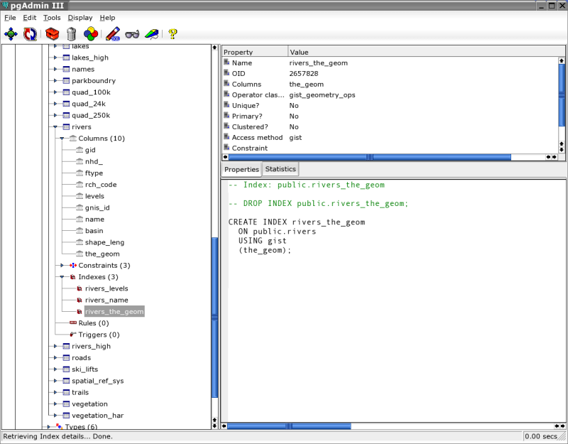
Figure 3: Screenshot of the graphical pgAdmin client with a session in a spatial database schema (Yosemite Park)
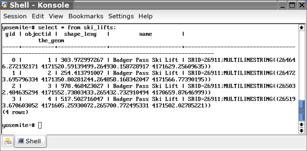
Figure 4: Screenshot of the text based psql client with a session in a spatial database schema (Yosemite Park)
Now that the spatial data has been imported, we have to work on a serverside extraction script. In this tutorial we use PHP for that purpose, but it is possible to use whatever serverside technology you are familiar with, as long as you generate the same SVG fragment structure. For this example a river layer is extracted, data is grouped and symbolized according to a level attribute. Additionally, the data is simplified with a Douglas-Poiker algorithm (Simplify()) and clipped (intersection()) for performance and bandwith saving reasons. To generate SVG geometry the AsSVG() function contributed by Klaus Förster is used.
The proposed workflow in example 3 is temporary. We think that at a later stage it would be more elegant to establish a XML language to desribe all the necessary layer parameters and to feed this description into the extraction script. This would eliminate the need to program a specific section for each individual layer to extract. This language could be similar to the UMN map file, but customized to the specific needs of SVG mapping applications. Watch for a newer project/tutorial covering such a map layer description.
Following is an example on how to extract data using PHP. The code will first be shown and then explained what it does. You may copy the example and change it to match your setup/parameters. For didactical reasons we only show the simplified code for one map layer. The example linked above has two map layers with nested svg structures.
<?
header("Content-type: text/xml");
//the content-type header is necessary for Mozilla SVG and the XMLHttpRequest
//specify connect variables
//test url: sendGeom.php?layername=hydrology&xmin=244000&ymin=4150000&xmax=308000&ymax=4231000×tamp=123
$username = 'webuser';
$dbGeomName = 'earth';
$password = 'svgextractor';
$hostname = 'pg.mydomain.com';
//get URL parameters
$layername = $_GET['layername'];
$myId = $layername.'_tempGeometry';
$xmin = intval($_GET['xmin']);
$xmax = intval($_GET['xmax']);
$ymin = intval($_GET['ymin']);
$ymax = intval($_GET['ymax']);
$timestamp = $_GET['timestamp'];
$width = $xmax - $xmin;
$height = $ymax - $ymin;
//set srid for UTM zone 11N, change that to match your epsg projection code
$srid = 26911;
//intersection polygon to clip out data where useful
$intersectPolygon = 'GeometryFromText(\'POLYGON(('.$xmin.' '.$ymin.','.$xmax.' '.$ymin.','.$xmax.' '.$ymax.','.$xmin.' '.$ymax.','.$xmin.' '.$ymin.'))\','.$srid.')';
//tolerance for generalization
$simplifyTolerance = $width / 800;
//connect to db
$my_pg_connect = pg_Connect('host='.$hostname.' dbname='.$dbGeomName.' user='.$username.' password='.$password) or die ('Can\'t connect to database '.$dbGeomName);
//case hydrology
if ($layername == 'hydrology') {
print '<g id="'.$myId.'" xmlns="https://www.w3.org/2000/svg" xmlns:attrib="https://www.carto.net/attrib" attrib:timestamp="'.$timestamp.'">'."\n";
//extract the rivers
print '<g id="'.$myId.'_rivers" fill="none" stroke="cornflowerblue" stroke-width="'.$width * 0.001.'">'."\n";
//first determine tablename and select criteria
//you could define multiple tablenames here, e.g. for multiple map scales,
//and switch them according to the $width variable
$tablename = 'rivers';
$addWhereClause = ' AND (type_name = \'Stream/Rriver\' OR type_name = \'Canal/Ditch\' OR type_name = \'Pipeline\')';
//now define threshold values for river levels
if ($width > 50000) {
$addWhereClause .= ' AND levels < 4';
}
elseif ($width <= 50000 and $width > 30000) {
$addWhereClause .= ' AND levels < 5';
}
elseif ($width <= 30000 and $width > 20000) {
$addWhereClause .= ' AND levels < 8';
}
elseif ($width <= 20000 and $width > 10000) {
$addWhereClause .= ' AND levels < 12';
}
elseif ($width <= 10000 and $width > 5000) {
$addWhereClause .= ' AND levels < 15';
}
else {
$addWhereClause .= '';
}
//sql parts:
$sql1 = 'SELECT name, levels, AsSVG(intersection(';
$sql2 = ','.$intersectPolygon.'),1,1) AS svg_geom FROM '.$tablename.' WHERE the_geom && setSRID(\'BOX3D('.$xmin.' '.$ymin.', '.$xmax.' '.$ymax.')\'::box3d,'.$srid.')';
$orderBy = ' ORDER BY levels ASC';
//distinquish between filtered and full resolution, concatenate sql
if ($width > 5000) {
$mySQL = $sql1.'Simplify(the_geom,'.$simplifyTolerance.')'.$sql2.$addWhereClause.$orderBy;
}
else {
$mySQL = $sql1.'the_geom'.$sql2.$addWhereClause.$addWhereClause.$orderBy;
}
//execute sql command
$my_result_set = pg_Exec($my_pg_connect, $mySQL) or die (pg_ErrorMessage());
//get number of rows retrieved
$numRecs = pg_NumRows($my_result_set);
$oldClass = '';
$i = 0;
while ($i < $numRecs) {
$resultArray = pg_Fetch_Array($my_result_set, $i);
//check if a new group is opened
if ($oldClass != $resultArray['levels']) {
//close group if already open
if ($oldClass != '') {
print "</g>\n";
}
//define stroke-width for new group
$strokeWidth = '';
if ($resultArray['levels'] < 4) {
$strokeWidth = 'stroke-width="'.$width * 0.003.'"';
}
elseif ($resultArray['levels'] >= 4 and $resultArray['levels'] < 5) {
$strokeWidth = 'stroke-width="'.$width * 0.0025.'"';
}
elseif ($resultArray['levels'] >= 5 and $resultArray['levels'] < 8) {
$strokeWidth = 'stroke-width="'.$width * 0.0020.'"';
}
elseif ($resultArray['levels'] >= 8 and $resultArray['levels'] < 15) {
$strokeWidth = 'stroke-width="'.$width * 0.0015.'"';
}
print '<g id="'.$tablename.'_'.$resultArray['levels'].'" '.$strokeWidth.'>'."\n";
$oldClass = $resultArray['levels'];
}
$mySvgString = $resultArray['svg_geom'];
//check if the returned element contains data
if (strlen($mySvgString) > 0) {
print "\t".'<path attrib:name="'.$resultArray['name'].'" d="'.$mySvgString.'" />'."\n";
}
$i++;
}
if ($numRecs > 0) {
print "</g>\n";
}
print "</g>\n";
print '<attrib:layerData id="'.$layername.'Data" attrib:nrRecs="'.$numRecs.'" attrib:layerName="'.$layername.'" />'."\n";
//close open group
print "</g>\n";
}
//close db connection
pg_Close($my_pg_connect);
?>
The first few lines define connection variables: user, databasename, password and hostname. For security reasons, it is recommend that a separate user with fewer access rights is defined for the purpose of extracting data in this php-extraction script. That user needs only have "select" rights on the tables you want to expose. Additionally, it needs "select" rights on the table containing the spatial reference information (spatial_ref_sys) and the table containg the geometry column information (geometry_columns).
The next few lines (after the comment "//get URL parameters") receive the information (parameters) from the URL string. The layername, the boundingbox (xmin, xmax, ymin, ymax) and a timestamp are needed. As a result of the bounding box parameters the map width ($width) can be calculated, which is an important variable for data filtering and symbolization options. The $srid variable holds the srid/epsg information. The same number used for converting/importing the GIS data (see example 2) has to be used, or else the queries won't work. The $intersectPolygon variable holds a string describing a clipping polygon that will be used later to clip the data. The $simplifyTolerance variable defines a filter tolerance used in the data reduction function Simplify() an implementation of the Douglas Poiker generalization algorithm.
Following, is the line executing the database connection based on the parameters specified previously. Next, a if statement branches according to the requested layername, in this case hydrology. In this example only one layer (hydrology), containing rivers, is used but in reality there would be multiple layers and sub-layers. Two or more physical database layers may form one nested SVG layer. For example imagine the hydrology layer containing line geometry (rivers), polygon geometry (lakes) and point geometry (cascades, waterfalls, springs, etc.). This can all be exposed as one logical layer. In the generated SVG fragment nested groups sharing common symbolization parameters would be received.
Within the "hydrology" if statement the first print statement opens a SVG <g> element. This group contains an unique id concatenated with the dynamic layername and the string "_tempGeometry". This naming convention needs to be followed to enable correct execution of the JavaScript which controlls the loading of data into the mapping client. Additionally, it contains a reference to the SVG namespace the data is within, a reference to a foreign namespace, which is used for the attribute data, and a timestamp, which is also needed by the clientside dataloading function. The reference to the SVG namespace is important, esp. for the current MozillaSVG implementation, that otherwise would not correctly append the SVG fragment. Nested in that group there is a subgroup for the rivers. This subgroup also has an id-attribute, that can be defined in anyway, but it needs to be unique. It is only used for descriptive reasons, e.g. reading the code manually. Styling information, such as fill and stroke is added as well. Note the use of the $width variable in the context of defining the stroke-width attribute. The stroke-width is defined as a percentage value of the current map-width. That way the line width will stay constant and independent of the selected scale factor.
The following if statement branches for two different table names. In this case a coarse table is used for larger map widths and a more detailed tables for smaller map extents. These tablenames need to match the tablenames in the Postgis database. The next if/elseif statement defines a sub selection based on the levels attributes. Larger map extents result in selections of only the major rivers, smaller map extens also load less important rivers.
Based on that information a SQL query string can be built. The first part contains all the attributes that wanted to be queried and the opening of the AsSVG() and intersection() command. The second part contains the tablename (FROM part) and the && operator (WHERE part) which is the "overlap" operator. If A's bounding box overlaps B's bounding box the operator returns true. Please note that this is the main operator that can currently benefit from the spatial index introduced before, hence it is strongly recommend to use this operator in your queries. The $orderBy variable indicates that is wanted to order the result using the levels attribute. This is necessary for the grouping of the individual records into one SVG group sharing common graphical attributes. The next if statement concatenates the individual SQL strings to one valid SQL command. We distinguish between larger map extents where we Simplify() the data and smaller map extents where the data isn't reduced. The second parameter of the Simplify() function is the simplify tolerance specified at the beginning of the script as a fraction of the current map extent. Increasing the tolerance results in smaller file sizes, but coarser geometry. Experiment with the tolerance values to get good compromizes between data quality and file sizes.
The AsSVG(the_geom,1,1) function potentially has three parameters: the first parameter is the column name containing the geometry, the optional second parameter specifies whether the output uses absolute or relative coordinates for the path geometry. If values with a lot of digits before the comma are used, relative coordinates are usually more compact. A value of 0 (default) means absolute coordinates, a value of 1 means relative coordinates. The optional third parameters specifies how many decimal places you want to use: 1 means that one decimal place after the comma is used. Please also note how several postgis functions are nested: in the inner part there is the geometry column_name. Around this there is the Simplify() function, around which is the intersection() function, around which the resulting geometry using the AsSVG() function is finally converted.
The following if statement distinguishes between fitered (simplified) and full resolution. Again, based on the map width. The final SQL string is concatenated, which is executed in the following line (pg_Exec()). The query result is saved in an array of associative arrays, called $my_result_set. To receive the number of selected records, use the pg_NumRows($my_result_set) function.
Next, there is a loop over all the records in the result set. The variable used as the loop end critera is $numRecs. The first line gives an extract of the result set - the current record. This record (an associative array) is saved in the array $resultArray. An individual element of a record can be extracted with the notation $resultArray['key'], where the key is the column name in the database.
The next if-statement checks if a new group has to be opened. This is the case if the last river level (stored in the variable $oldClass is different from the current river level. In this case, a new group is opened and new "stroke-width" values are set. Again, in relation to the current map width. The line $mySvgString = $resultArray['svg_geom']; retrieves the actual SVG geometry, already in the format of the d-attribute required for the SVG <path /> element. If the stringlength (strlen) is larger than 1 (not an empty string) a new path-element is written out. As a non-graphical attribute, attrib:name is written out, containing the river's name.
Finally, a custom element in our "attrib" namespace is created, containing layerdata, in this case only the number of retrieved records. This information can be used in the SVG application to give feedback on how many elements have been loaded. In the next line the group is closed, and finally the database connection is closed with the command pg_Close($my_pg_connect);.
After editing the file sendGeom.php and eliminating the errors, the script should be tested manually first, before it is integrated with the SVG application:
Type in the following address in your browser (change the parameters to match your project: server, path, layername and min/max values):
server.yourdomain.org/projectDirectory/sendGeom.php?layername=hydrology&xmin=244000&ymin=4150000&xmax=308000&ymax=4231000×tamp=123
As a result, you should receive a correctly structured SVG fragment that should validate in a XML validator if you add the correct header information.
Next, the SVG application needs to be enhanced to allow for dynamic data-loading
You can start from the example provided at the end of the OGC/WMS tutorial. Download the following files involved in the project and adapt the links to the external linked javascript files (at the beginning of the svg-file after the svg-root element):
Open the file index.svg (previous example4.svg) in a text or XML editor and go to the mainMap section. Add a new empty group called hydrology after the path element of the park boundary. Add as many groups as you have dynamic map layers:
<g id="hydrology" visibility="visible" />
In the function init() add the following two lines after the line var dynamicLayers = new Array();:
dynamicLayers["hydrology"] = {"key":"hydrology","value":"yes","loaded":"no"};
dynamicLayers.push(dynamicLayers["hydrology"]);
This adds a new entry in the associative array dynamicLayers which holds data on dynamic layers to be loaded with getURL() or XMLHttpRequest. The "key" attribute is the layername, the "value" attribute defines whether a layer should be loaded and the "loaded" attribute defines whether a layer is already loaded or not.
A timestamp needs to be added to the myMainMap object in order to control the data loading better, in case the user zooms or pans very fast, i.e. faster than the data he is requesting arrives. When the getURL() is triggered, the sendGeom.php is sent to the current timestamp as a parameter. Every time the user pans or zooms, the timestamp is updated. If the user pans or zooms before the previously requested data arrives, data is not added to the document tree, but simply dropped. Data is only added to the DOM tree when it matches the current timestamp. In the function loadProjectSpecific() (file index.svg) add the following lines:
//generate timestamp
var now = new Date();
myMainMap.timestamp = now.getTime();
The property "timestamp" of the "myMainMap" object now holds the current date and time (expressed in milli-seconds since January 1, 1970) and is updated each time the user zooms and pan. While still in the function loadProjectSpecific(), add another line that will trigger the dynamic data loading. Add it just before the function getOrthoImage():
//get vector layers
getLayers();
To enable data loading, five additional JavaScript functions are needed. Place them in the script section of the file "index.svg" after the last function, or alternatively in an external js file:
//get layers, calls function getSingleLayer() for each individual layer
function getLayers() {
//loop over all entries in the myMainMap.dynamicLayers array
for (i=0;i<myMainMap.dynamicLayers.length;i++) {
//see if layer is switched on
if (myMainMap.dynamicLayers[i].value == "yes") {
//at first dynamic layer add a new nrLayerToLoad/timestamp entry
if (myMainMap.nrLayerToLoad[myMainMap.timestamp.toString()]) {
//at second or further layer increment the nrLayerToLoad variable
myMainMap.nrLayerToLoad[myMainMap.timestamp.toString()]++;
}
else {
//start a new entry for this timestamp
myMainMap.nrLayerToLoad[myMainMap.timestamp.toString()] = 1;
}
//call getSingleLayer() which makes the individual network requests
getSingleLayer(myMainMap.dynamicLayers[i].key);
//set visibility of loadData text
if (myMainMap.nrLayerToLoad[myMainMap.timestamp.toString()] == 1) {
document.getElementById("loadingData").setAttributeNS(null,"visibility","visible");
}
}
}
}
//get a single layer
//this function makes the actual network requests using either getURL() or XMLHttpRequest()
function getSingleLayer(layerId) {
//build a url string
var myUrlString = "sendGeom.php?layername="+layerId+"&xmin="+myMainMap.curxOrig+"&ymin="+((myMainMap.curyOrig + myMainMap.curHeight)* -1)+"&xmax="+(myMainMap.curxOrig+myMainMap.curWidth)+"&ymax="+(myMainMap.curyOrig * -1)+"×tamp="+myMainMap.timestamp;
//call getURL() if available
if (window.getURL) {
getURL(myUrlString,addGeomGetURL);
}
//call XMLHttpRequest() if available
else if (window.XMLHttpRequest) {
//this nested function is used to make XMLHttpRequest threadsafe
//(subsequent calls would not override the state of the request and can use the variable/object context of the parent function)
//this idea is borrowed from https://www.xml.com/cs/user/view/cs_msg/2815 (brockweaver)
function XMLHttpRequestCallback() {
if (xmlRequest.readyState == 4) {
if (xmlRequest.status == 200) {
//parse and import the SVG fragment
var importedNode = document.importNode(xmlRequest.responseXML.documentElement,true);
//call function addGeom
addGeom(importedNode);
}
}
}
var xmlRequest = null;
xmlRequest = new XMLHttpRequest();
xmlRequest.open("GET",myUrlString,true);
xmlRequest.onreadystatechange = XMLHttpRequestCallback;
xmlRequest.send(null);
}
//write an error message if either method is not available
else {
alert("your browser/svg viewer neither supports window.getURL nor window.XMLHttpRequest!");
}
}
//this function is only necessary for getURL()
function addGeomGetURL(data) {
//check if data has a success property
if (data.success) {
//parse content of the XML format to the variable "node"
var node = parseXML(data.content, document);
addGeom(node.firstChild);
}
else {
alert("something went wrong with dynamic loading of geometry!");
}
}
//add the geometry to the application
//note that empty groups in the main-map have to exist
function addGeom(node) {
//extract id of the layer
var curDynLayer = node.getAttributeNS(null,"id").replace(/_tempGeometry/,"");
//extract timestamp
var timestamp = parseInt(node.getAttributeNS(attribNS,"timestamp"));
//compare current timestamp with timestamp of the node data
if (timestamp == myMainMap.timestamp) {
var myGeometryToAdd = document.getElementById(curDynLayer);
//remove previous content
if (myMainMap.dynamicLayers[curDynLayer].loaded == "yes") {
var tempGeometry = document.getElementById(curDynLayer+"_tempGeometry");
myGeometryToAdd.removeChild(tempGeometry);
}
//append new content
myGeometryToAdd.appendChild(node);
//set loaded flag to "yes"
myMainMap.dynamicLayers[curDynLayer].loaded = "yes";
}
//decrement layers to load
myMainMap.nrLayerToLoad[myMainMap.timestamp.toString()]--;
//set loadData text to hidden after last layer was loaded
if (myMainMap.nrLayerToLoad[myMainMap.timestamp.toString()] == 0) {
document.getElementById("loadingData").setAttributeNS(null,"visibility","hidden");
}
}
The function getLayers() loops over all dynamicLayers (a property (array) of the myMainMap object). If the "value" of the current dynamicLayer is set to "yes", a new URL is built to request new data. Before that URL is sent, we check if an entry of our current timestamp exists in the myMainMap.nrLayerToLoad array. This array holds the number of layers to load for the current timestamp. If a value does not exist in the array for the current time stamp, a new entry is created. In case it already exists (e.g. if there are more than one dynamic layers), this value is incremented. If three dynamic layers need to be loaded, the value of myMainMap.nrLayerToLoad[myMainMap.timestamp.toString()] will be three. Next, we test whether the value is one, in which case a visible text element has to be made, indicating "loading data". The URL string contains the call to sendGeom.php with all necessary parameters, such as layername, bounding box and the current timestamp. These parameters are extracted from the myMainMap instance of the map object documented at Navigation Tools for SVG Maps. Depending on the remote call method available, either the method getURL() or the method XMLHttpRequest calls the php file on the server which extracts the data and sends it back to the client. The callback functions addGeomGetURL(data) (in case of getURL() method) or XMLHttpRequestCallback() (in case of XMLHttpRequestCallback() method) receive the data from the server and forward it to the function addGeom which removes previous content and appends the new content to the DOM tree.
Let us explain in a few sentences the differences between the two approaches for getting additional data: .getURL is not part of the SVG specification, but it is available as a proprietary extension in ASV3, ASV6 and the current Batik version. It only allows asynchronous remote calls, which means that after the remote call, the script execution continues and does not wait until the data is received. Data is later received by a separate callback function. In our case this is the preferred method anyway. getURL does not have a progress event and does not allow to cancel remote calls. While getURL is purely a procedural method, XMLHttpRequest is based on an object and offers additional methods and properties. The use of getURL() is very simple: one single call getURL(myUrlString,addGeomGetURL); issues the request and specifies the callback function. XMLHttpRequest was first introduced by Microsoft as an ActiveX extension and is meanwhile implemented in all major browsers, such as Firefox, Safari, Opera and Konqueror. It is also not a W3C standard, but the recommended way to do remote calls until the DOM3 W3C methods are implemented in the browsers. XMLHttpRequest allows to receive ResponseHeader data and provides additional status properties for data loading, including a progress event. It also allows to do synchronous remote calls and allows to cancel remote calls. Because this method is more powerful than the getURL() method it is also a little bit more complex to use. We first need to create a new object instance of the XMLHttpRequest object, next we need to open a connection to a URL, register a callback function and finally do the .send(null) request. As with getURL, a callback function receives the data. This callback function is registered to the onreadystatechange event of the XMLHttpRequest object. Since this method is object based and we don't want to add many global objects we need to ensure that this method is threadsafe over several concurrent remote calls. One solution for this problem is to embed the callback function as an "inner function" in the function that makes the remote call. This way, the object and variable context is maintained and not lost after subsequently calling the same callback method. (see www.xml.com/cs/user/view/cs_msg/2815 A threadsafe implementation of XMLHttpRequest). To make the decision which of the two remote call methods should be used, the script tests for the availability of the methods: if (window.getURL) { ... } else if (window.XMLHttpRequest) { ... } else { alert("errormessage") }. To get more information on getURL() and XMLHttpRequest see the following resources: jibbering.com/2002/5/dynamic-update-svg.html Dynamically updating SVG based on serverside information by Jim Ley, Dynamic HTML and XML: The XMLHttpRequest Object by Apple and XMLHttpRequest by XULPlanet.
The callback functions receive the data as described above. Within the callback function addGeomGetURL(data) we check if the "data" object (which contains the data received from the server) has a property called data.success. If it doesn't have one, it means that something went wrong with the data loading, e.g. a bad web server response code (e.g. missing file)). We can continue, if the "data.success" property exists. The XML content is parsed from the data.content property using the parseXML() method available in ASV and Batik. Finally, the function addGeom(node.firstChild) is called with the first child of the DOCUMENT_FRAGMENT_NODE received through parseXML() as an argument. In our case this first child is the first group element within the documentFragment node. Alternatively, if you use XMLHttpRequest, the other callback function XMLHttpRequestCallback() is used. This callback function is called whenever the readyState changes. In our case we are only interested in readyState 4, which is triggered after the transaction is complete. In that case we use the property responseXML which contains the received XML fragment, import the documentElement of this fragment using .importNode(fragment,true) and hand it over to the function addGeom() for further actions. In that context it is important to note that the serverside script needs to send the correct content-type header: see second line in script sendGeom.php (header("Content-type: text/xml");. Otherwise the property responseXML would not work.
Within the function addGeom the "id" attribute is extracted from the first group child of the node, using the getAttributeNS(null,"id") method. The "_tempGeometry" part of the string is replaced, so that only the layername is received. Next, the timestamp attribute is extracted and compared with the current timestamp. If the received data is old (which is the case if the user zooms or pans faster than the data download lasts), the data packet is ignored. If the timestamp is up-to-date, the node content is appended to the layer group. Prior to appending the node, the old content must be deleted if it existed. After appending the node, the "loaded" variable of the current dynamicLayer is set to yes, which indicates that the layer was received. Finally, the nrLayerToLoad[myMainMap.timestamp.toString()] variable is decremented and if the value zero is reached, the visibility of our "data loading ..." text element can be turned off. All elements are now loaded. The function addGeom(data) is run for every dynamicLayer to load. Since data loading works asynchronly there is no guarantee that the returned data arrives in the same order that the requests where made.
The user needs to be given feedback while the data is being loaded. For that purpose, a group element with the id "loadingData" is created, whose visibility is turned on while the application is loading data and turned off after all data has arrived. Add the following lines above the main map (below in the order in the file/DOM tree):
<!-- Loading Data Status -->
<g id="loadingData" visibility="hidden">
	<rect x="200" y="300" width="150" height="35" fill="white" fill-opacity="0.8"/>
	<text x="275" y="325" class="allText subtitleText centerText">Loading Data ...</text>
</g>
Right now your project should be running. Put your project files including the sendGeom.php script on your webserver and start the project from there. It is important that the sendGeom.php is located on the same server where the index.svg file is loaded from, otherwise the getURL() function won't work. This is a security restriction, inherent in all browsers and plugins.
To make the prototype fully functional we still need to add a new checkbox and modify the toggleMapLayer scritp. Add the following linein the init() function of your index.svg file, after the third checkBox ("DOQ") to add a new checkBox element. Please refer to the checkbox_and_radiobutton tutorial for details:
myMapApp.checkBoxes["hydrology"] = new checkBox("hydrology","checkBoxes",200,60,"checkBoxRect","checkBoxCross",true,"Hydrology",labeltextStyles,12,6,undefined,toggleMapLayer);
To extend the toggleMapLayer function, add the following lines after the first if-block. This tells the scripting logic not to load the dynamic layer hydrology next time the map extent is changed.
       else {
            if (id == "hydrology") {
                   myMainMap.dynamicLayers[id].value = "no";
             }
       }
and the following lines within the lower if-block starting with if (checkStatus) {:
         if (id == "hydrology") {
             myMainMap.dynamicLayers[id].value = "yes";
             if (myMainMap.nrLayerToLoad[myMainMap.timestamp.toString()]) {
                  myMainMap.nrLayerToLoad[myMainMap.timestamp.toString()]++;
             }
             else {
                  myMainMap.nrLayerToLoad[myMainMap.timestamp.toString()] = 1;
             }
             document.getElementById("loadingData").setAttributeNS(null,"visibility","visible");
             getSingleLayer(id);
         }
This sets the value of myMainMap.dynamicLayers["hydrology"] to yes, sets the visibility to "visible" and fetches the additional data.
For a fully validating XML/SVG file, the SVG DTD still needs to be extended to allow the GIS attributes and metadata in the foreign namespace. To do this, replace the second line in the file "index.svg" containing the DOCTYPE declaration with the following construct:
<!DOCTYPE svg PUBLIC "-//W3C//DTD SVG 1.1//EN" "https://www.w3.org/Graphics/SVG/1.1/DTD/svg11.dtd" [
<!ATTLIST svg
	xmlns:attrib CDATA #IMPLIED
>
<!ATTLIST path
	attrib:name CDATA #IMPLIED
>
<!ATTLIST g
	attrib:timestamp CDATA #IMPLIED
>
<!ENTITY % SVG.g.extra.content "|attrib:layerData">
<!ELEMENT attrib:layerData EMPTY>
<!ATTLIST attrib:layerData
	id CDATA #IMPLIED
	attrib:nrRecs CDATA #IMPLIED
	attrib:layerName CDATA #IMPLIED
>
]>
Now, at the end of this tutorial you should have a functional, validating SVG mapping application that can load dynamic SVG data from a Postgis database. This example illustrates how your example should look like, at the end of the tutorial. In this example application not only the rivers are loaded, but also the lakes and water river areas, all nested in within the hydrology layer. Additionally, a landcover layer is loaded.
During more complex SVG projects, such as this project, one regularly runs into errors and developing problems. The following tricks can help during development:
Often, people developing SVG GIS or mapping apps complain that SVG is slow. However, if you follow certain guidelines you can enhance the perfomance to a satisfying speed:
If you have any feedback regarding this tutorial, corrections or suggestions for improvements, please contact the authors. Good luck with your own SVG mapping projects!
| Last modified:
Tuesday, 10-Dec-2019 21:37:57 CET
© carto:net (andreas neumann & andré m. winter) original URL for reference: https://old.carto.net/papers/svg/postgis_geturl_xmlhttprequest/index.shtml |